Fault Diagnostics & Cyber-Security for a Spacecraft Attitude System

Overview

In the MSc course Fault Diagnostics and Security for Control Systems (4DM110, Q4 2025–2026) at TU Eindhoven, I designed and evaluated a stack of diagnostic and cyber-defence methods for a three-axis spacecraft attitude determination system. A spacecraft closes its control loop over a radio link that is shared, open to eavesdropping, and exposed to two very different threats: faults (a gyro that develops a bias, a reaction wheel that delivers the wrong torque) and deliberate cyber-attacks (an adversary corrupting the data crossing the network — possibly in a way a classical detector never sees).

The project works through three increasingly adversarial layers on the same plant — the published spacecraft model of Pirmoradi et al.:

Fault diagnostics (T1–T2) — an unknown-input observer (UIO) that detects and reconstructs sensor faults from the output residual.
Secure state estimation (T3) — a multi-observer estimator that reconstructs the true state when an unknown sensor is under attack, with a sharp structural finding about when it works and when it cannot.
Resilient control (T4) — the nonlinear-encoding defence of Joo, Qu and Namerikawa (2021), which uses two synchronised chaotic circuits to make a perfectly stealthy integrity attack visible at zero performance cost.

Project Report — Fault Diagnostics and Estimation of a Spacecraft Attitude Determination System

Download

System and model

From nonlinear rigid body to decoupled double integrators

The spacecraft has three rate gyroscopes measuring the body rates $(p, q, r)$ and three vector sensors measuring the attitude angles $(\phi, \theta, \psi)$ , actuated by three reaction-wheel torques. Euler's rigid-body equations are nonlinear because of the gyroscopic coupling between axes, but around the stationary operating point $x = 0$ , $u = 0$ the gyroscopic cross-products vanish and the small-angle kinematics give $\dot\phi \approx p$ . The six states decouple into three identical double integrators:

\dot{x} = A_c x + B_c u,\qquad A_c=\begin{bmatrix}0_{3\times3}&0_{3\times3}\\ I_3&0_{3\times3}\end{bmatrix},\qquad C_c = I_6,

with state $x = [\,p\ q\ r\ \phi\ \theta\ \psi\,]^\top$ , input the reaction-wheel torques, and full-state measurement ( $C = I_6$ , three gyros + three vector sensors). The moments of inertia are $I_x = 10$ , $I_y = 12$ , $I_z = 2~\mathrm{kg\,m^2}$ .

Output-feedback PD controller

The open-loop plant has six poles at the origin — in space there is no natural damping, so any disturbance makes the attitude drift. A decentralised PD law $u = -Kx$ stabilises each axis. Matching the per-axis characteristic polynomial $s^2 + \tfrac{K_d}{I}s + \tfrac{K_p}{I}$ to the canonical $s^2 + 2\zeta\omega_n s + \omega_n^2$ gives

K_p = \omega_n^2\, I,\qquad K_d = 2\zeta\omega_n\, I.

Scaling each gain by its axis inertia cancels the $1/I$ in $B_c$ , so a single choice of $\omega_n = 0.1~\mathrm{rad/s}$ and $\zeta = 0.8$ gives identical closed-loop behaviour on all three axes regardless of inertia — about $1.5\%$ overshoot and a $\pm 2\%$ settling time near $38$ s.

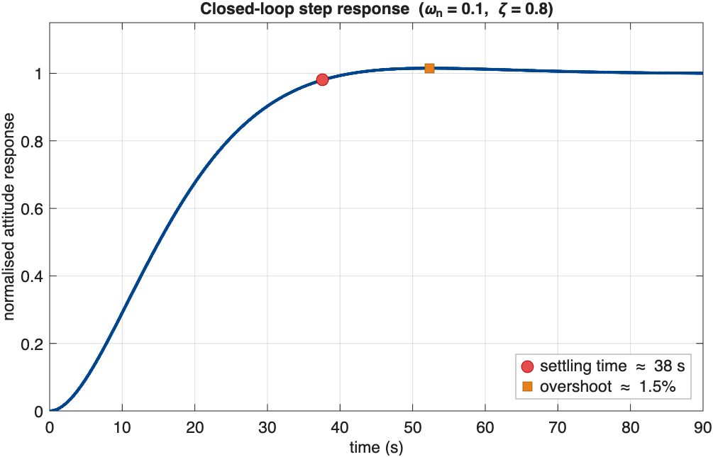
Closed-loop step responses for the roll, pitch and yaw axes under the decentralised PD law with (omega_n, zeta) = (0.1, 0.8). All three axes track the same second-order response, settling to within plus or minus 2 percent in roughly 38 seconds with about 1.5 percent overshoot. — Closed-loop step response per axis for $(\omega_n, \zeta) = (0.1, 0.8)$ . Inertia-scaled gains make all three axes track the same second-order response.

Discretisation — exploiting a nilpotent $A_c$

The estimators run on a digital computer, so the model is discretised with a zero-order hold at $T_s = 0.1$ s. The key shortcut is that $A_c$ is nilpotent ( $A_c^2 = 0$ ), so the matrix exponential and the ZOH integral both terminate after two terms — the discretisation is exact, and ZOH and Tustin happen to coincide:

A_d = I_6 + A_c T_s,\qquad B_d = \Big(I_6 T_s + \tfrac{1}{2}A_c T_s^2\Big) B_c,\qquad A_{cl} = A_d - B_d K.

The closed-loop $A_{cl}$ has spectral radius $|z| \approx 0.992 < 1$ , so the discrete loop is Schur stable — a fact the fault diagnostics exploit directly.

Tasks 1–2 — Fault diagnostics with an unknown-input observer

Fault model

A sensor fault is an unknown input $a(k)$ that corrupts the measurement without touching the physical motion. So the fault never enters the dynamics ( $B_{\text{fault}} = 0$ ) and appears only at the output, where each affected channel contributes a unit column to $D_{\text{fault}}$ :

x(k+1) = A_{cl}\,x(k),\qquad y(k) = x(k) + D_{\text{fault}}\,a(k).

Because each broken sensor adds an independent column to $D_{\text{fault}}$ , the stacked fault matrix always keeps full column rank — so any combination of simultaneous sensor faults is, in principle, separable.

The UIO that collapses to a physics simulator

A general unknown-input observer reconstructs the state from a window of outputs and recovers the fault from the residual,

\hat a(k) = \begin{bmatrix} B_{\text{fault}} \\ D_{\text{fault}} \end{bmatrix}^{+} \begin{bmatrix} \hat x(k+1) - A_{cl}\hat x(k) \\ y(k) - C\hat x(k) \end{bmatrix}.

For this spacecraft three simplifications collapse the full design to almost nothing. Sensor faults appear instantly in the measurement, so no look-ahead window is needed ( $L = 0$ ). There is no actuator-path disturbance to decouple, so the decoupling matrix $S = 0$ . And because the PD loop has already made $A_{cl}$ Schur, no observer feedback is needed, so $G = 0$ . Together:

F = S + GN = 0,\qquad E = A_{cl},\qquad \Rightarrow\quad \hat x(k+1) = A_{cl}\,\hat x(k).

The "observer" becomes a pure physics simulation of the healthy closed-loop model, deliberately blind to the sensors. Any divergence in the residual $y(k) - \hat x(k)$ is then read directly as a fault on the corresponding channel.

Scenario 1, a 0.3 degree-per-second bias injected on the pitch gyro at t = 40 seconds. Top panel: the noisy measurement diverges upward while the UIO state estimate stays on the true, healthy pitch-rate trajectory. Bottom panel: the reconstructed fault estimate jumps from zero and locks onto the 0.3 degree-per-second bias within one or two samples, with a steady-state RMSE of 0.051 degrees per second, equal to the gyro noise floor. 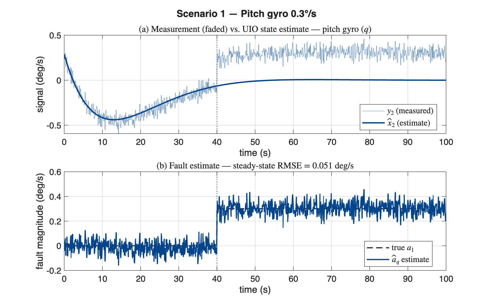— Scenario 1 — pitch-gyro fault ( $+0.3^\circ/\mathrm{s}$ at $t = 40$ s). The reconstructed fault $\hat a$ locks onto the true bias within a sample or two; steady-state RMSE of $0.051^\circ/\mathrm{s}$ sits exactly at the sensor noise floor, so the estimator adds no bias of its own.

Across all scenarios — single gyro fault, single angle-sensor fault, and two simultaneous faults (yaw gyro + pitch sensor) — the reconstructed $\hat a$ followed each injected bias within one to two samples, with steady-state RMSE at the noise floor on every channel.

Robustness to inertia uncertainty

Since the diagnostic runs on a model built from the inertias $I_x, I_y, I_z$ , a TA question prompted a robustness study: what if the true inertia drifts, $I^{\text{true}} = (1+\delta)\,I^{\text{nom}}$ ? Because the gains scale as $K \propto I$ while $B_d \propto 1/I$ , the product $B_d K$ is nominally inertia-independent, so the closed loop barely moves. Sweeping $\delta$ from $-60\%$ to $+60\%$ , the worst-case fault-free residual grows with $|\delta|$ but never crosses the detection threshold $\mu$ — inertia uncertainty alone does not raise a false alarm.

Two panels showing robustness to an inertia error delta swept from minus 60 to plus 60 percent. Left: closed-loop step responses remain stable for every delta; a heavier spacecraft (positive delta) overshoots more, up to about 8 percent at plus 60 percent, while a lighter spacecraft is overdamped, but all settle to the reference. Right: the worst-case fault-free residual rises with the magnitude of delta but stays below the detection threshold mu across the whole sweep. 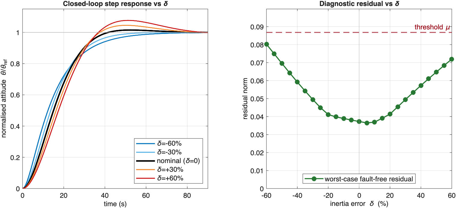— Robustness to inertia error $\delta \in [-60\%, +60\%]$ . Left: the loop stays stable and always settles. Right: the worst-case fault-free residual rises with $|\delta|$ but never crosses the alarm threshold $\mu$ .

Task 3 — Secure state estimation under sensor attacks

Task 3 raises the adversary: now an unknown sensor is being actively attacked, and the estimator must reconstruct the true state without knowing which one. The model adds a per-sensor attack signal,

x(k+1) = A_d x(k) + B u(k),\qquad y_i(k) = C_i x(k) + a_i(k),

and we defend against a single attacked sensor ( $M = 1$ ). The reason for $M = 1$ is itself a finding — for $M = 2$ no two-sensor subset of this six-state plant is observable, so the algorithm is infeasible.

Observer bank and decoder

The secure estimator (Chong–Wakaiki–Hespanha, 2015) runs a bank of Luenberger observers over sensor subsets and trusts the one that is most self-consistent. For every $S$ of $N - M = 5$ sensors it runs a level-1 observer, and for every $P$ of $N - 2M = 4$ sensors a level-2 cross-check. The decoder scores each level-1 subset by its worst disagreement with its own sub-observers, then selects the minimum:

\pi_S(k) = \max_{P \subset S,\,|P| = N-2M} \big\|\hat x_S(k) - \hat x_P(k)\big\|, \qquad \sigma(k) = \arg\min_{|S| = N-M} \pi_S(k), \qquad \hat x(k) = \hat x_{\sigma(k)}(k).

A clean subset excludes the attacked sensor, so its observer converges and scores $\pi_S \approx 0$ ; an attacked subset disagrees with its sub-observers and scores high. The least-disagreeing subset is the trustworthy estimate.

The headline finding — rate decodes, angle doesn't

The catch is observability. Theorem 1 requires every $(N - 2M)$ -sensor subset $(A_d, C_J)$ to be observable. Checking all $\binom{6}{4} = 15$ subsets in MATLAB, only three are observable. The reason is structural: each axis is a $[\text{rate}, \text{angle}]^\top$ pair, and $\dot\theta = \omega$ means you can recover a rate from an angle, but not an angle from a rate alone (you'd need the integration constant). So a subset is observable if and only if it keeps all three angle sensors $\{4, 5, 6\}$ :

\{1,4,5,6\},\qquad \{2,4,5,6\},\qquad \{3,4,5,6\}.

This splits the defence cleanly in two:

Attack a rate gyro (sensors 1–3) → it can be dropped while keeping all angle sensors → an observable hypothesis exists → the decoder isolates it correctly. ✅
Attack an angle sensor (sensors 4–6) → every observable subset is forced to keep all three angle sensors → no subset can exclude the corrupted one → the decoder is fooled. ❌

A deterministic bias sweep confirmed this is structural, not noise- or magnitude-dependent: rate-sensor attacks decode correctly from $0.05$ to $10^\circ/\mathrm{s}$ , while a roll-angle attack is decoded wrong from $0.5$ to $90^\circ$ .

Failure case: a bias injected on the roll angle sensor (sensor 4) at t = 40 seconds. Top: the level-1 disagreement scores for the exclude-1, exclude-2 and exclude-3 observers all spike after the attack; none stays near zero. Middle: the decoded subset never selects exclude-4 (the true attacked sensor, marked by the red dashed line) because every subset that drops an angle sensor is unobservable and excluded from the candidate pool. Bottom: on the roll channel the secure estimate tracks the corrupted measurement and diverges from the true state. 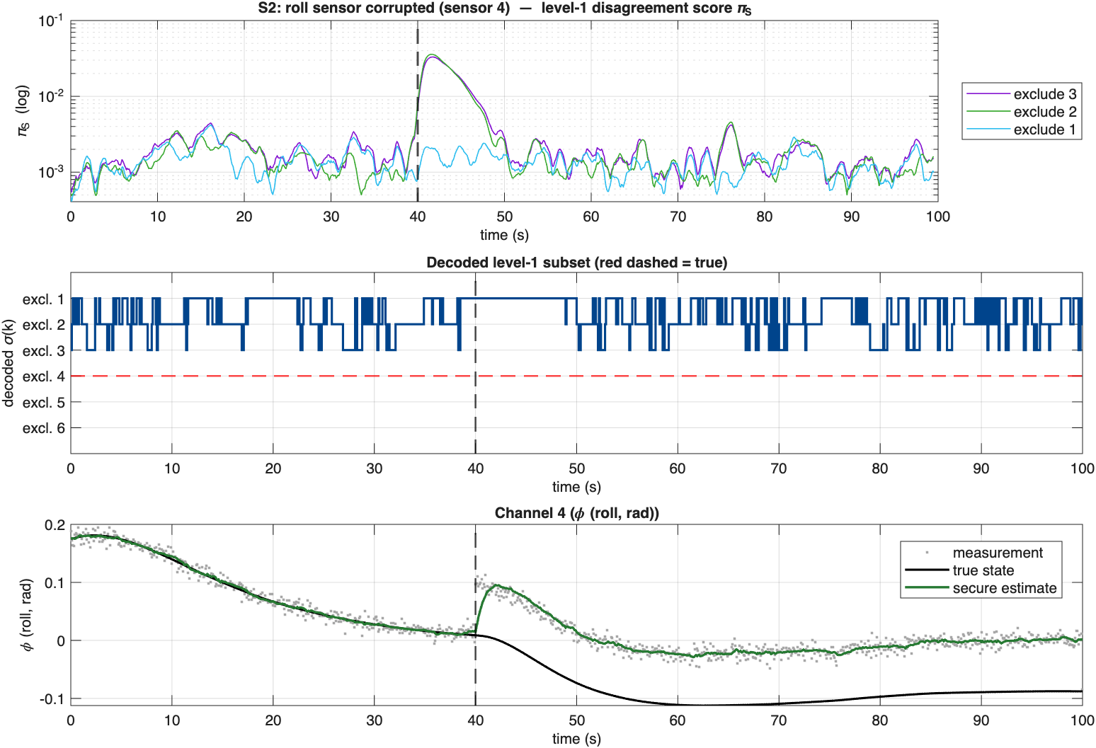— Failure mode — roll-angle-sensor attack (sensor 4). The true subset would have to *exclude* sensor 4 (red dashed), but that hypothesis is unobservable and never enters the candidate pool, so the decoder picks a wrong subset and the secure estimate (green) follows the attack instead of the true state (black).

Restoring one-fault observability

The blind spot is fixable: it exists because dropping an angle sensor unobserves its axis. Adding redundant cross-axis "summation" sensors that measure linear combinations of two angles each,

y_7 = \phi + \theta,\qquad y_8 = \theta + \psi,\qquad y_9 = \phi + \psi,

closes a linearly independent cycle over the attitude angles, so a missing angle can always be reconstructed from the others. With $N = 9$ , every one of the $\binom{9}{7} = 36$ subsets becomes observable — the system is now globally one-fault observable. (I also worked through a compact $6 \times 6$ variant that hits the same rank condition without adding any sensors — at the cost of coupling rate and angle into the same channel.)

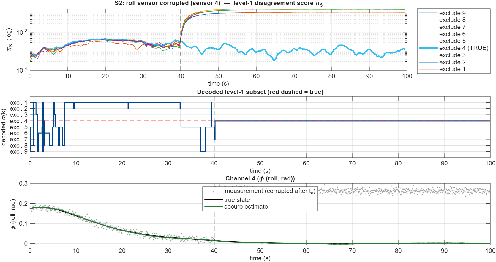
The same roll angle sensor attack, now with the augmented nine-sensor architecture including the three summation sensors. The decoder correctly identifies and rejects the corrupted roll sensor, and the secure state estimate stays locked on the true roll trajectory throughout the attack, confirming global one-fault observability. — The same roll-angle attack with the augmented $N = 9$ summation-sensor architecture: the decoder now rejects the corrupted sensor and the secure estimate stays clean — the angle-sensor blind spot is resolved.

Try it yourself. The demo below runs the full multi-observer estimator live in your browser — the exact algorithm, observability test, and decoder described above. Attack a rate gyro (sensors 1–3) and the decoder isolates it; attack an angle sensor (4–6) and watch the secure estimate get dragged off the truth — then tick Add redundant summation sensors and watch the same attack get rejected. Nothing about the rate/angle split is hard-coded; it emerges from which sensor subsets are observable.

Decoder: ✓ tracking true stateobservable subsets: 0 level-1 / 0 level-2

What to watch: You're attacking sensor 4 (Roll angle, an angle sensor) with only the original 6 sensors. Every observable subset must keep all three angle sensors, so none can exclude the attacked one: no score reaches the floor and the secure estimate is dragged toward the corrupted measurement. This is the observability blind spot — now tick "Add redundant summation sensors" below and watch it recover.

Attack which sensor?

Angle-sensor attacks (red) sit in the observability blind spot — unless you add redundant sensors below.

Attack bias: 5.0 °Attack activeAdd redundant summation sensors (N = 9)

Live simulation. Top: the level-1 disagreement score $\pi_S$ for every observable subset (log scale) — a clean subset drops toward zero. Bottom: the true state, the secure estimate, and the noisy (possibly attacked) measurement on the targeted channel. Attack an angle sensor and watch the estimate get dragged off the truth — then tick the redundant-sensor box and watch it recover.

Task 4 — Resilient control against stealthy integrity attacks

Task 3's angle-sensor attack was effectively a stealthy attack — it lived in an observability blind spot and a passive estimator never saw it. Task 4 implements an active defence from Joo, Qu and Namerikawa (2021): the goal is to make a perfectly stealthy attack visible, at zero performance cost when there is no attack. As in the paper, this layer is studied in continuous time.

The perfectly stealthy attack

An attacker who knows the dynamics can match the closed-loop model ( $K_a = K$ , $H = 0$ ) and inject a sensor signal that exactly cancels the physical effect of its own actuator tampering in the residual:

u_a = -K x_a + r_a,\qquad \dot x_a = A_c x_a + B_c u_a,\qquad y_a = -C_c x_a.

Against a classical residual-based detector this is invisible — the residual stays flat while the spacecraft is driven off course.

Nonlinear encoding and decoding

The defence multiplies the control signal by a fast, chaotic modulation factor before it crosses the network, and divides it back out at the plant:

u_{tx} = (1 + \varepsilon\hat\xi)(-K\hat x),\qquad u_{rx} = \frac{u_{tx} + u_a}{1 + \varepsilon\xi},\qquad \varepsilon|\hat\xi| \le 0.5,

where $\xi$ is the plant's chaotic signal and $\hat\xi$ the controller's synchronised copy. The bound $\varepsilon|\hat\xi| \le 0.5$ keeps the denominator in $[0.5, 1.5]$ so it never divides by zero; the encoding depth is $\varepsilon = 0.15$ . When the two circuits are synchronised ( $\hat\xi = \xi$ ) and there is no attack, the factors cancel exactly and the plant receives precisely $-K\hat x$ — zero performance cost. But an attacker cannot reproduce $\xi$ , so an injected $u_a$ is scaled by an uncancellable chaotic factor and forced into the residual. This gives the clean detection guarantee

z_a = 0 \iff u_a = 0.

Chaos from Chua's circuit

The secret signal $\xi$ comes from a Chua circuit running the canonical double-scroll attractor, with its piecewise-linear negative-resistor diode

g(v) = m_1 v + \tfrac{1}{2}(m_0 - m_1)\big(|v + B_p| - |v - B_p|\big),\quad m_0 = -\tfrac{8}{7},\ m_1 = -\tfrac{5}{7},\ B_p = 1.

A master circuit on the plant generates $\xi = v_1$ ; a slave on the controller side sees only the scalar $v_1$ and locks onto it through a Pecora–Carroll coupling term (gain $l_c = 8$ ). Joo's Lemma 2 guarantees the slave's tracking error decays exponentially once $l_c$ exceeds a threshold ( $\approx 2.14$ here), so $\hat\xi \to \xi$ — verified in simulation below.

Master and slave Chua-circuit synchronisation. Top panel: the master encoding signal xi and the slave's copy overlap almost perfectly within a fraction of a second. Bottom panel: the synchronisation error, the absolute difference between master and slave, plotted on a log scale, drops below ten to the minus two within about 0.3 seconds and keeps decaying with periodic dips toward ten to the minus six. 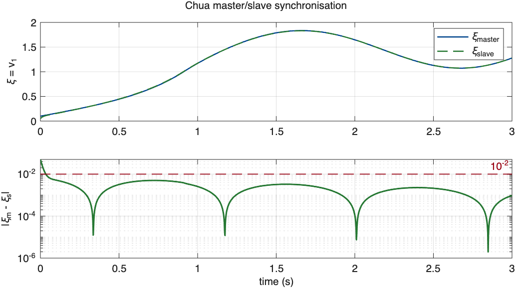— Pecora–Carroll synchronisation of the two Chua circuits. The slave locks onto the master within a fraction of a second (error below $10^{-2}$ by $\approx 0.3$ s), so $\hat\xi \approx \xi$ and the encoding cancels cleanly under no attack.

Catching the attack T3 missed

With the encoding switched on, the same stealthy attack that the classical detector never sees jumps the residual decisively above the alarm threshold $\mu$ at the instant of injection — while the no-attack response is identical with encoding on or off, confirming there is no performance penalty. Crucially, the encoded detector catches a roll-angle attack — the exact attack class that lived in Task 3's observability blind spot. The two deliverables are complementary: passive secure estimation and active nonlinear encoding cover each other's gaps.

Three stacked panels comparing the detector with encoding off versus on. Top: the residual norm on a log scale. With encoding off (classical detector) it stays flat at the noise floor before and after the attack at t = 40 seconds. With encoding on it jumps several orders of magnitude above the threshold mu the moment the attack starts. Middle: the attitude angle theta drifts and wraps around either way, illustrating that detection is not prevention. Bottom: the controller's state estimate is driven away from zero during the attack, showing the controller is deceived even though the attack is now detectable. 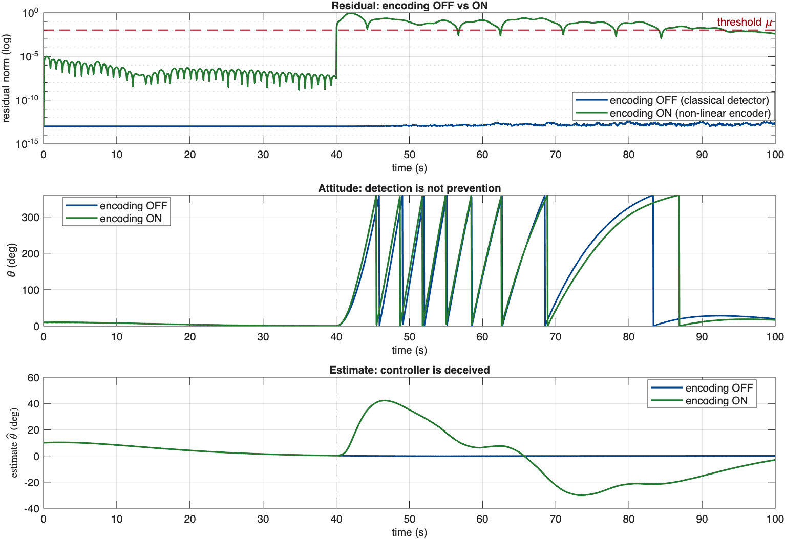— Encoding off vs on. The classical residual (blue) never moves; the encoded residual (green) leaps above the threshold $\mu$ at injection ( $t = 40$ s). With no attack the two responses are identical — detection costs nothing. Note the middle panel: *detection is not prevention* — the attack is revealed, but still drives the spacecraft off course.

Try it yourself

The simulation below runs the same continuous-time implementation in your browser — the full 3-axis attitude loop, the twin Chua circuits, and Joo's Lemma-1 attacker, integrated live with RK4. Launch the attack and watch the encoded residual leap eleven decades at the injection instant while the classical detector never moves. Two honest details to notice: the attacker's internal model self-stabilises ( $u_a \to 0$ ), so the encoded residual decays back after firing — the alarm therefore latches at the first crossing, exactly like a real intrusion alert. And detection is not prevention: the bottom panel shows the true pitch being dragged toward $r_a/K_p \approx 2865°$ while the deceived estimate stays put. Untick the attack to watch the controller recover once the sensor mask disappears.

No attack — encoded and classical loops identical (zero performance cost)t = 0 s · |ξ − ξ̂| = 1.0e+0

Encoding depth ε = 0.15Launch stealthy attack

speed

Live simulation — a faithful port of the course MATLAB (spacecraft_encoding_continuous.m): the full 3-axis attitude loop, Joo et al.'s Lemma-1 self-stabilising attacker, and the twin Chua circuits with the paper's coupling (Lemma 2, l_c = 8). Left: the master circuit tracing the double-scroll attractor that generates the shared secret ξ. Top right: the detector residual with encoding off (classical, blue) vs on (encoded, green) — under the same perfectly-stealthy attack the classical residual sits at the numerical floor while the encoded one leaps 11 decades at onset. Because the attacker's model self-settles (u_a → 0), the encoded residual decays back after firing — so the alarm latches at the first crossing. Bottom right: detection is not prevention — the true pitch (orange) is dragged away toward r_a/K_p ≈ 2865° while the deceived estimate (teal) never moves. Untick the attack to watch the controller recover.

A sweep over the encoding depth $\varepsilon$ confirmed the design trade-off: deeper encoding raises the peak residual and shrinks the detection delay (down to $\approx 0.05$ s), with $\varepsilon = 0.15$ sitting comfortably in the fast-detection region while respecting the $\varepsilon|\hat\xi| \le 0.5$ safety bound. The closed loop also remained input-to-state stable — the peak attitude deviation grows linearly with the attack magnitude $r_a$ , giving an operator a predictable window to respond.

Results & Reflections

This was the most adversarially-minded controls project I have done, and the through-line was honest negative results. The secure state estimator does not simply "work" — it works for rate-sensor attacks and provably fails for angle-sensor attacks, and chasing down exactly why (the open-loop $\dot\theta = \omega$ observability structure, not noise or tuning) was more instructive than a clean success would have been. Reporting that failure sharply, then designing the redundant-sensor architecture that fixes it, turned a limitation into the most interesting part of the work.

The three layers also taught me how differently faults and cyber-attacks have to be treated. A fault shows up in the residual by construction, so a collapsed UIO — literally a healthy-model simulation — suffices. A stealthy attack is engineered to be invisible to exactly that residual, so the only defence is to inject a secret the attacker cannot reproduce. Watching two chaotic circuits synchronise and then quietly cancel — leaving the loop untouched until the moment an attacker tries to hide inside it — was the most elegant idea in the course. And the recurring caveat, detection is not prevention, is a good reminder that the estimator's job is to tell the operator the truth, not to save the spacecraft on its own.

Technologies Used

MATLAB (place, obsv, expm, c2d, ode45, exportgraphics), unknown-input observer design, Luenberger multi-observer banks, secure state estimation (Chong–Wakaiki–Hespanha), observability analysis over sensor subsets, nonlinear chaotic encoding (Joo et al. 2021), Chua-circuit chaos and Pecora–Carroll synchronisation, Lyapunov / ISS stability arguments, LaTeX