Control Engineering: Fourth-Order Motion Setup

Overview

PATO fourth-order motion setup

In this project, my partner and I designed and implemented a feedback and feedforward control system for a fourth-order PATO motion setup — a two-mass spring-damper system representative of the dynamics found in semiconductor lithography and high-speed printing. The primary objective was to achieve the fastest possible scanning motion over a 120-radian stroke while maintaining the lowest tracking error on the non-collocated (end-effector) side.

The project was conducted as part of the Control Engineering course at TU Eindhoven (Group 67, with Kayden Knapik) and written in IEEE conference format.

Full Report — Control Engineering: Fourth-Order Motion Setup

Download

System Identification

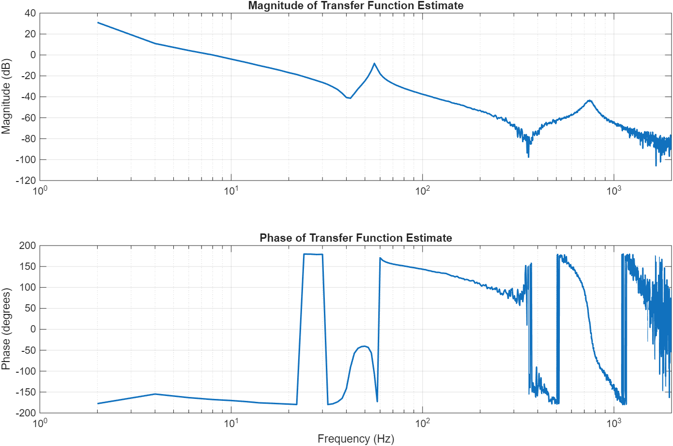
Before designing a controller, we performed frequency-domain system identification using a 3-point measurement technique. Broadband noise was injected into the plant, and three signals were recorded simultaneously: the disturbance, the plant input, and the plant output. This allowed us to compute an accurate open-loop FRF even under closed-loop conditions.

The Frequency Response Function was estimated using Welch's method with a Hanning window and 50% overlap:

H(f) = \frac{S_{dy}(f)}{S_{du}(f)}

where $S_{dy}$ is the cross-power spectral density between the disturbance and output, and $S_{du}$ is the cross-power spectral density between the disturbance and input.

The plant exhibits two distinct transfer functions:

Collocated (motor-side encoder): contains an anti-resonance/resonance pair
Non-collocated (end-effector): fourth-order roll-off with resonance only

Bode plot of the identified collocated system, showing the anti-resonance/resonance pair characteristic of motor-side feedback. — Collocated $H_c(s)$ — note the anti-resonance dip preceding each resonance peak.

Bode plot of the identified non-collocated system, with the same resonance peaks but no anti-resonance — what the controller actually has to deal with for end-effector tracking. — Non-collocated $H_{nc}(s)$ — fourth-order roll-off, no anti-resonance.

Controller Design

Feedforward

Feedforward was designed to handle the bulk of reference tracking, with three components tuned sequentially:

Coulomb friction gain ( $K_{fc}$ ) — matched deceleration/acceleration errors
Viscous friction gain ( $K_{fv}$ ) — minimized constant-velocity error
Acceleration feedforward ( $K_{fa}$ ) — eliminated remaining error peaks

This reduced peak tracking error from 1.4 rad to 0.1 rad.

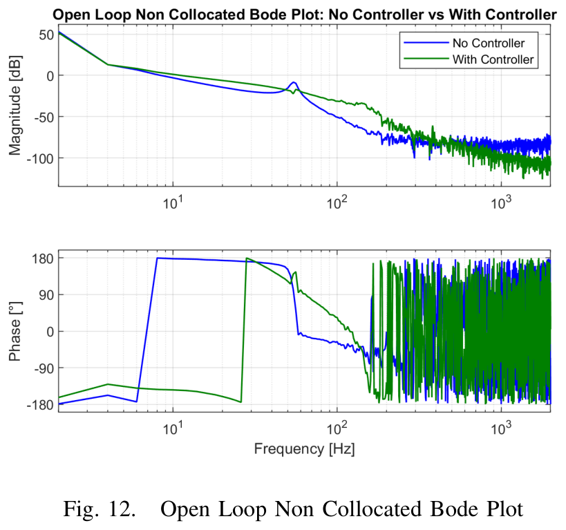
Feedback (Loop Shaping)

The feedback controller was designed using classical loop-shaping:

Component	Parameters
Proportional Gain	2.5
Notch Filter (60 Hz)	Zero damping: 0.01, Pole damping: 0.7
Notch Filter (3.45 Hz)	Zero damping: 0.1, Pole damping: 0.001
Lead-Lag Filter	Zero: 14 Hz, Pole: 60 Hz
2nd Order Low-Pass	Pole: 200 Hz, Damping: 0.2

The 60 Hz notch targeted the main resonance frequency, while the 3.45 Hz notch addressed a low-frequency mode caused by non-ideal mechanical coupling. The lead filter provided phase margin around the crossover frequency.

Results

The final controller achieved Region I performance:

RMS Tracking Error: 2.252 mrad (requirement: < 6 mrad)
Peak Tracking Error: 9.425 mrad (requirement: < 12 mrad)
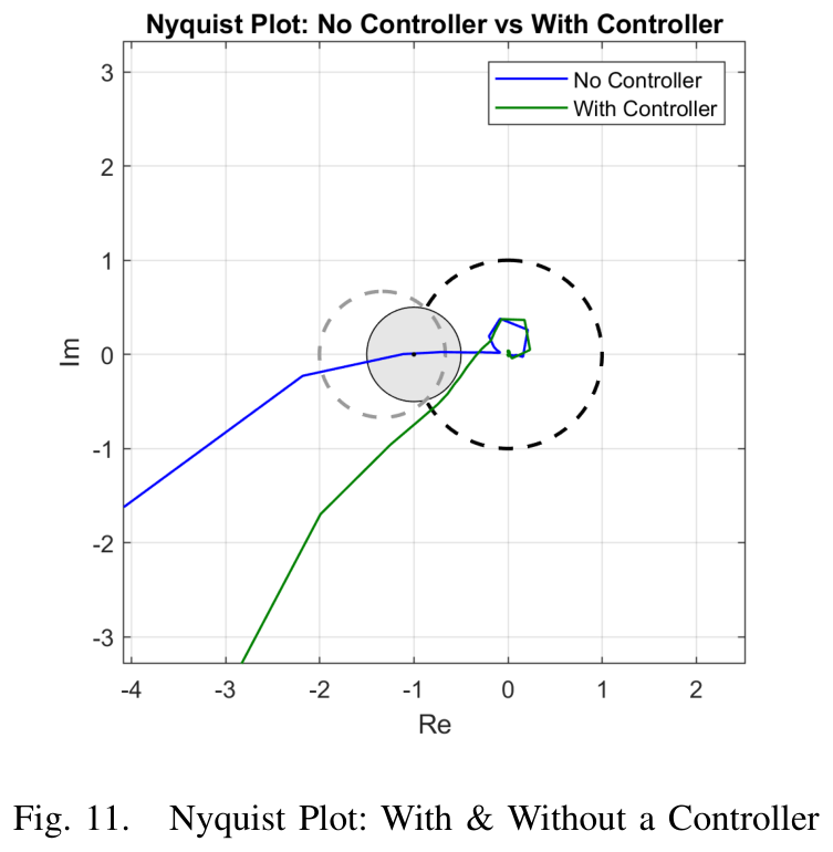
Sensitivity margin ( $\|S(j\omega)\|$ ): below 6 dB

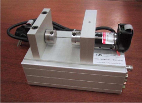
The system was validated on real hardware (Raspberry Pi-based real-time controller connected to the physical PATO setup), with Bode plots, Nyquist diagrams, and power spectral density analysis confirming stability and performance.

Open-loop non-collocated Bode plot with and without the synthesized controller, showing the notch dips at the targeted resonance frequencies and the high-frequency roll-off from the second-order low-pass. — Open-loop $L(j\omega) = C(j\omega) H_{nc}(j\omega)$ . The notches at 3.45 Hz and 60 Hz cleanly carve out the problem modes.

Nyquist plot of the loop gain with and without the controller. The controlled loop stays outside the modulus-margin circle around the −1 critical point. — Nyquist with the modulus-margin circle (≤ 6 dB) — the controlled loop never enters it.

Results & Discussion

This project deepened my understanding of frequency-domain control design — from the subtleties of FRF measurement (coherence, spectral leakage) to the practical trade-offs of loop shaping (bandwidth vs. noise amplification). Tuning feedforward before feedback proved to be a powerful design philosophy that I've since applied in other projects.

Technologies Used

MATLAB, Simulink, Raspberry Pi (real-time control), physical PATO motion setup, IEEE LaTeX template