Overview
In the MSc course Multibody and Nonlinear Dynamics (4DM10, Q2 2025–2026) at TU Eindhoven, I completed two substantial take-home assignments. The first assignment covers multibody dynamics — deriving a constrained DAE model of a floating telescopic crane and simulating its forced response. The second covers nonlinear dynamics — passivity-based energy-tracking control of an oscillating mass on a rolling ring, plus a Lyapunov stability analysis of a COVID-25 SIR epidemic model with vaccination.
Assignment 1 — Floating Telescopic Crane
The first assignment models an offshore floating telescopic crane — the kind used for heavy-lift construction — as a planar constrained multibody system. The schematic on the left of the thumbnail shows the three rigid bodies (boat, rotary arm, telescopic rod with a point-mass load) together with the buoyancy spring-damper pair, the cable spring , the rotary motor , and the prismatic actuator force .
System and coordinates

The system uses the full redundant coordinate set
With 9 generalized coordinates and 5 holonomic scleronomic constraints (one translational for the boat, a revolute joint coupling body 1 to body 2, and a prismatic joint coupling body 2 to body 3), the system has 4 degrees of freedom. The coordinates are therefore dependent and call for the Lagrange-multiplier formulation.
Problem 1 — Model derivation
Following the standard Lagrangian workflow, I derived:
- Constraint equations for the three joints (2 equations from the revolute pair, 2 from the prismatic pair, 1 from the boat translation lock).
- Kinetic energy — including the cross-coupling term from the point-mass load rigidly fixed at the rod tip.
- Potential energy — gravitational plus the three elastic terms (buoyancy at each hull point, cable , and internal telescopic spring ).
- Non-conservative generalized forces — wave forces , motor torque , prismatic force , and the two viscous dampers .
- Equations of motion in the standard DAE form
With four independent motions and two applied inputs ( and ), the system is underactuated — the wave-induced sway and heave of the boat cannot be driven directly, only compensated for through the rotary joint.
Problem 1.7 — Forward dynamic simulation
Given the parameter table, the piecewise inputs
plus sinusoidal wave forces
and ,
I integrated the index-3 DAE with MATLAB's ode15s (stiff solver) over
s. Baumgarte stabilization (with manually tuned
, ) added to the second-derivative form of the constraint
equations kept constraint drift within
throughout the full 300-second simulation — essential at these actuator
magnitudes (–), where naive integration drifts in seconds.
Problem 2 — Simplified linear dynamics & FRF
For Problem 2 the rod and arm were rigidly fused (no telescoping), reducing the system to the minimal coordinate set . With and the wave forces set to zero, the nonlinear equations of motion reduce to three coupled ODEs (equations 7a–7c of the assignment), which I linearized around the equilibrium
to obtain . The eigenvalues of the linearized second-order system all had negative real parts, confirming local asymptotic stability of the operating point. The three undamped eigenmodes correspond to the heave mode (buoyancy spring), the boat-tilt mode, and the arm mode, and their eigenvectors clearly separate vertical from rotational motion at the low-frequency end of the spectrum.
The frequency response function from actuator torque to boat heave was then computed analytically from the linearized matrices:
with the low-frequency slope explained by compliance of the buoyancy spring and the two resonance peaks lining up with the computed eigenfrequencies.
Problem 2.3 — Inverse dynamics for wave compensation
Given measured boat motion and , the task was to reconstruct the torque that would generate exactly this motion on the physical system (an inverse-dynamics problem). Substituting the measured trajectory and its analytical derivatives into equation 7b directly yields with no integration required — a clean demonstration of the inverse-dynamic property of a reference trajectory for a smooth multibody system.
Assignment 2 — Nonlinear Dynamics
Assignment 2 split into two independent problems, both showcasing classical nonlinear-dynamics tools.
Problem 1 — Passivity-based energy control of an oscillating mass on a ring
A uniform ring (mass , inner radius , outer radius ) rolls without slipping on a flat surface. A point mass is mounted inside the ring, connected to the center via two identical springs of stiffness and rest length , free to slide along a body-fixed radial axis. An actuator applies a force on the point mass along that same axis, with reaction forces on each ring-contact point. The independent coordinates are
where is the ring-rotation angle and is the signed mass displacement from the ring center.
After deriving the Euler–Lagrange equations and expressing the total mechanical energy
the key observation is that differentiating along the flow yields
so the system is passive from input to output . That one line makes an energy-shaping control law available immediately.
The Lyapunov-based energy-tracking controller
The assignment asks us to design a feedback law that drives to a prescribed target energy . Using the Lyapunov candidate
the derivative along the flow is . Choosing the control law
yields , giving convergence to the invariant set . By LaSalle's invariance principle, trajectories either converge to the desired energy level or to an equilibrium with zero mass oscillation — no linearization, no feedback linearization, just passivity + Lyapunov.
Numerical exploration (Problem 1.5)
Simulating the closed loop with , kg, kg, m, m, N/m showed three distinct asymptotic regimes depending on :
| Regime | Asymptotic behavior |
|---|---|
| System settles at (target unreachable) | |
| Ring oscillates about bottom equilibrium | |
| Ring rotates indefinitely — enough energy to escape |
The threshold is the potential barrier (energy needed to lift the point mass to the top of the ring) — a clean physical interpretation of a bifurcation in an otherwise abstract Lyapunov analysis.
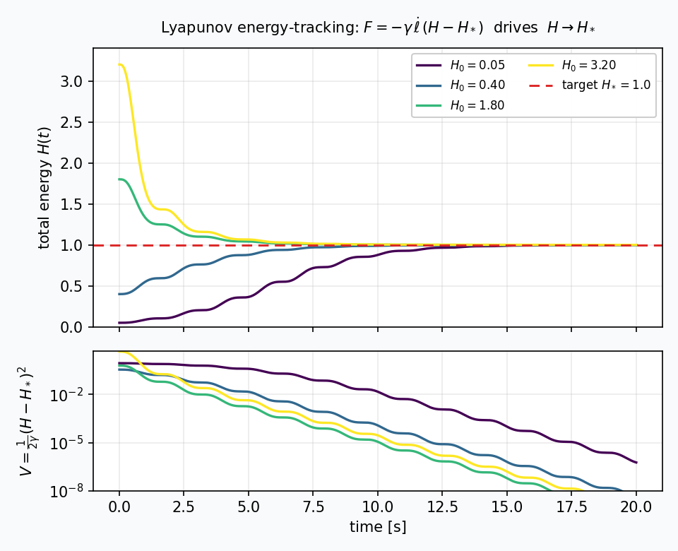
Energy-tracking simulation on a 1-DOF surrogate (). Top: converges to for four different initial energies. Bottom: the Lyapunov candidate decays monotonically (log-scale) — exactly the behavior LaSalle's principle guarantees.
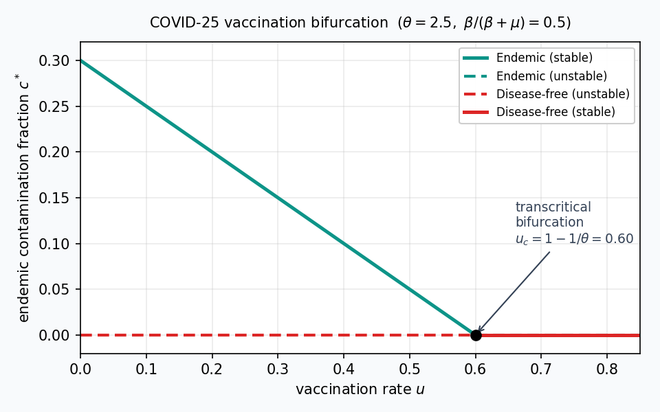
Problem 2 — COVID-25: SIR dynamics, stability, and vaccination
The second problem treats a population split into vulnerable (), contaminated (), and immune () compartments of constant total . After normalization to fractions , , , the reduced state-space model becomes
with . The set is forward-invariant (each boundary face is crossed inward by the vector field), so the reduced model suffices.
Equilibria and the epidemic threshold
Introducing the dimensionless group
the equilibria are the disease-free point and — when — the endemic point . Linearization classifies the disease-free equilibrium as a stable node for and a saddle for . The endemic equilibrium's global asymptotic stability for is proven using the radially unbounded Lyapunov candidate
whose time derivative reduces to after the algebraic identity .
Vaccination control & bifurcation
Adding a vaccination rate that sends a fraction of newborns directly from vulnerable to immune modifies the vulnerable equation to . With a 90%-efficient vaccine, the required vaccination rate to eliminate the endemic equilibrium works out to ; with a 100%-efficient vaccine the bifurcation occurs cleanly at . Plotting vs. gives a transcritical bifurcation diagram where the endemic branch collapses into the disease-free one exactly at the predicted .
Results & Reflections
These two assignments were the most mathematically demanding course work of Q2. The multibody assignment taught me how Baumgarte stabilization quietly saves a naive DAE solver from constraint drift — without it, the crane simulation diverges within seconds under -magnitude loads. The nonlinear assignment was a reminder that passivity arguments are often shorter than the linearized analysis they replace: one line of completely determines a globally stabilizing control law, where a linearized design would leave large regions of state space uncovered. The epidemiological half of Assignment 2 was a welcome change of domain — same Lyapunov toolkit, different physical interpretation.
Technologies Used
MATLAB (ode15s, symbolic toolbox, solve, vpa), Lagrangian mechanics
with multipliers, Baumgarte constraint stabilization, passivity-based control,
LaSalle's invariance principle, bifurcation analysis, frequency response
analysis