Overview
This project was completed individually for 4CM120 — Data-Based Optimization of Control Systems (TU Eindhoven, MSc Mechanical Engineering, Feb–Apr 2026). Taught by Dr.ir. Thijs van Keulen and Dr.ir. Leroy Hazeleger, the course studies real-time, model-free optimization for high-tech mechatronic systems.
The problem — nanometer-scale localization of a moving stage with respect to a reference frame — is directly relevant to atomic force microscopes and lithography machines, where fast and accurate alignment is critical. The approach implemented here is based on the patent by Van Keulen et al. (2021, Method of controlling a position of a first object relative to a second object, PCT/EP2020/070979).
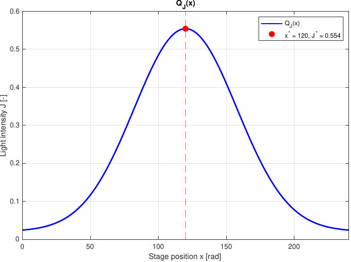
The objective function is the light intensity measured by a photodiode on the moving body as it passes under a fixed reference lens:
This Gaussian has a unique maximum at with . The goal of the ESC controller is to find this peak without any analytical model of — using only the measured intensity signal .
The Assignment
The project is split into two deliverables — both embedded below:
The Plant Model
The moving stage uses a combination of feedforward and feedback control to follow a reference position . The underlying fourth-order transfer function from input force to position is:
with a PD + second-order Low-Pass feedback controller:
where , , , . The full loop runs discrete-time at via zero-order-hold discretization.
Part I — Classical ESC in Simulation (Assignment 1)
How Extremum Seeking Control Works
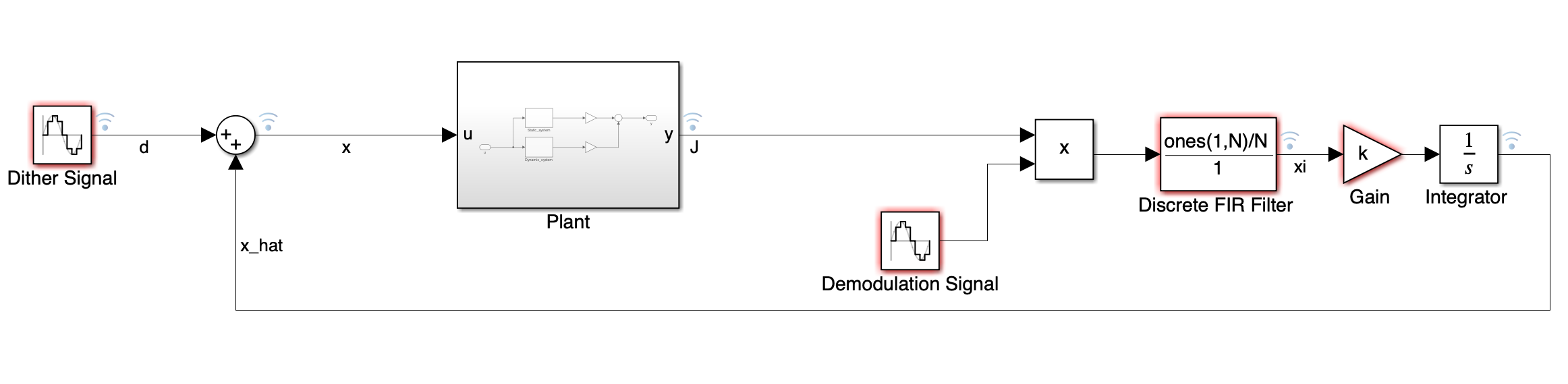
ESC estimates the gradient of the unknown objective by injecting a sinusoidal dither signal onto the reference. The measured output is then demodulated (multiplied by the same cosine) and filtered to extract the gradient component . An integrator uses this estimate to steer the nominal position toward the optimum.
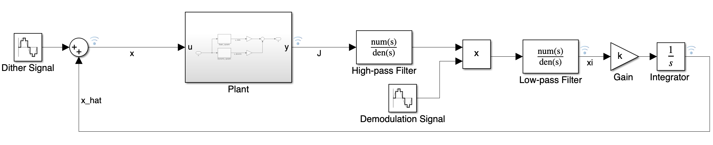
The loop has five elements:
- Dither signal — added to
- High-pass filter — removes DC
- Demodulation — multiplication by extracts gradient information
- Low-pass filter — smooths the estimate
- Integrator with gain — drives toward increasing
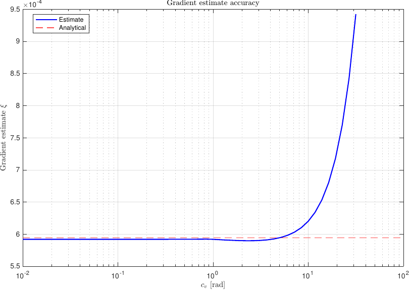
A critical design constraint is the timescale separation: .

Tuned values from Q2 placed on a log-frequency axis. The filter cutoff sits below the dither (so HP/LP can extract DC), and both sit well below the closed-loop bandwidth (so the plant looks like a static map at ).
Unimodality Assumption (Q1)
For ESC to converge to the global optimum from any initial condition , the objective function must be unimodal — i.e., have a single critical point. Since is Gaussian, and causes strict monotonic decrease in both directions. Only one zero of the gradient exists at , so the assumption is satisfied.
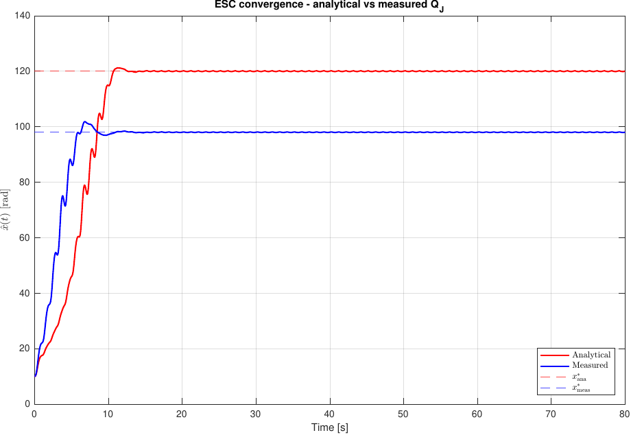
Optimal Parameters on the Static Map (Q2)
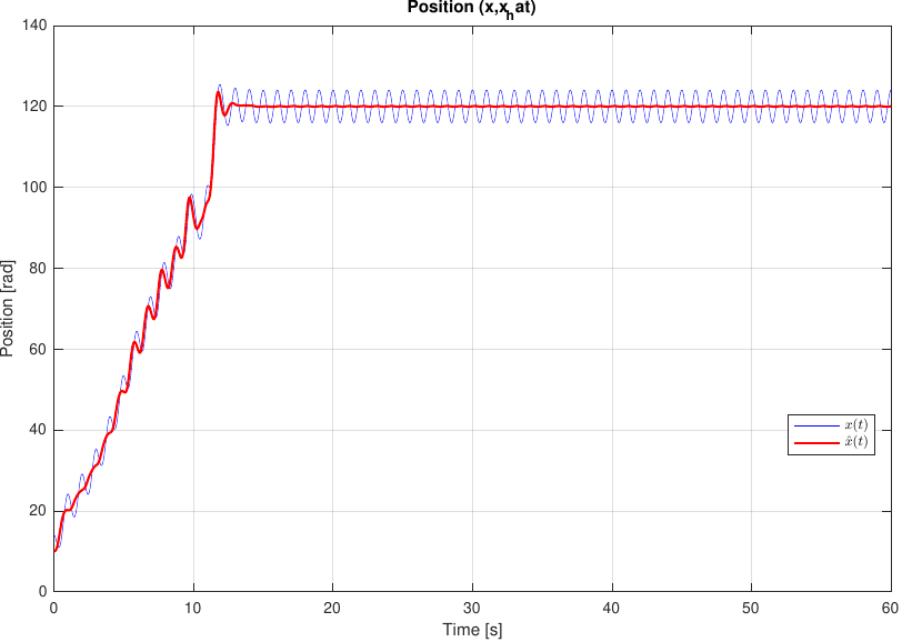
Starting from with prescribed, tuning converged on:
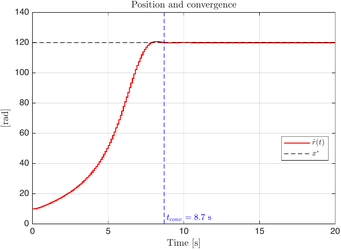
- Convergence time: 17.3 s
- Steady-state error: < 0.1 rad
- Peak intensity reached:
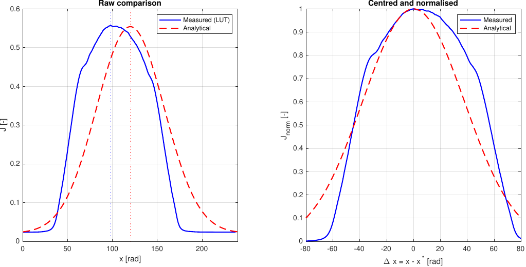
Measured vs. Analytical Objective (Q3)
The analytical was replaced with an experimentally measured objective function obtained by sweeping the stage slowly past the photodiode. Intensity values were binned into 0.5 rad intervals and averaged, producing a lookup table for Simulink interpolation.
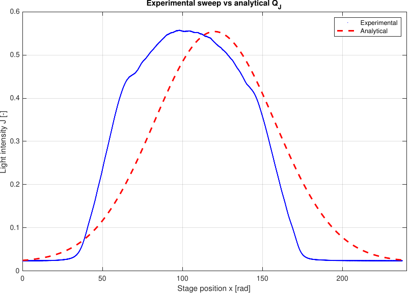
Key differences:
- Peak offset: the experimental peak appears at rather than — an encoder-zero offset
- Steeper slopes: the real lens-photodiode geometry produces sharper gradients near the peak
- The analytical parameters caused divergence on the measured objective because the high filter cutoff created phase lag through the steeper gradient
Re-tuning for the measured case required a lower filter cutoff () and slightly adjusted gains (, ).
Lookup Table vs Analytical Function (Q3)
Incorporating Plant Dynamics (Q5–Q7)
So far the plant was treated as a static map. In reality the moving stage has non-trivial dynamics: for ESC to work, the dynamic system must behave as a static map at the dither frequency — i.e., the closed-loop transfer function must satisfy:
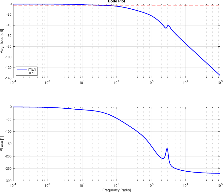
The Bode plot confirms a closed-loop bandwidth of . At the 1 Hz dither frequency (), and — well within the static-map regime.
With dynamics and noise enabled (disturbances = true, dynamics = true), the ESC was re-calibrated:
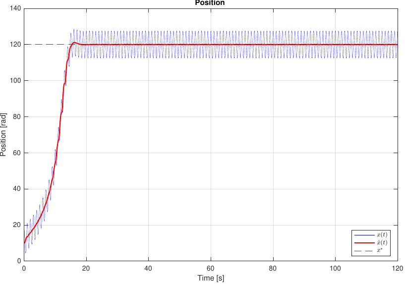
Despite the new constraints (phase lag, stage resonances, tighter filter speeds), convergence was achieved in ~20.8 s with all requirements met.
Part II — ESC on Physical Hardware (Assignment 2)
Assignment 2 took the simulation framework and deployed it on the real test setup — a motorized rotary stage with a photodiode. Three distinct ESC architectures were compared, both in simulation and on hardware:
- Classical ESC — sinusoidal dither with HP/LP filters
- Moving Average ESC — replaces the HP/LP filters with an exact moving average
- Sampled-Data ESC — discrete step perturbations with finite-difference gradients
Classical ESC on Hardware (C-Q1)
The Q7 simulation parameters were used as a starting point. Four experimental runs were performed on the physical setup.
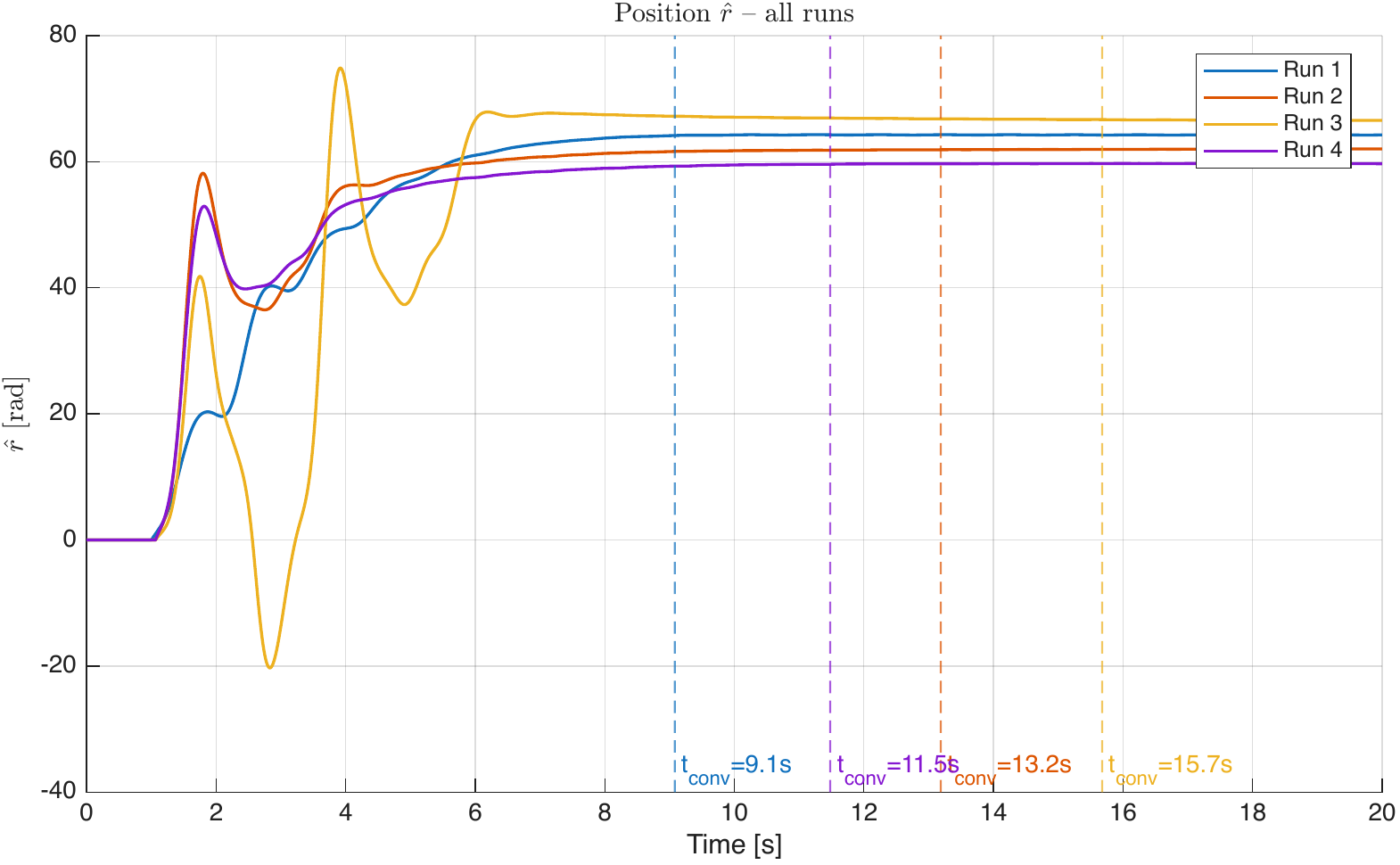
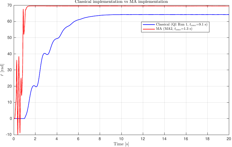
The best run matched the Assignment 1 Q7 parameters exactly and converged in 9.1 s — over a second faster than the simulation (10.6 s), due to the steeper real gradient.
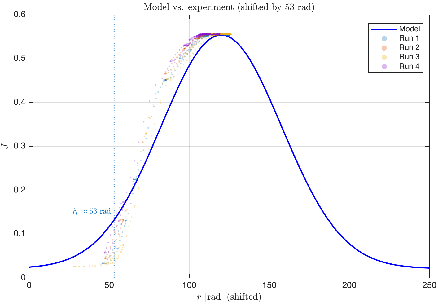
Encoder Offset Discovery
The physical encoder's zero position did not match the model's . The system converged to rather than the model's 120 rad, but the peak intensities were identical (). Aligning the data with a ~53 rad offset confirmed the experimental shape follows the model Gaussian near the peak but with steeper slopes further out.
Simulation vs. Experiment
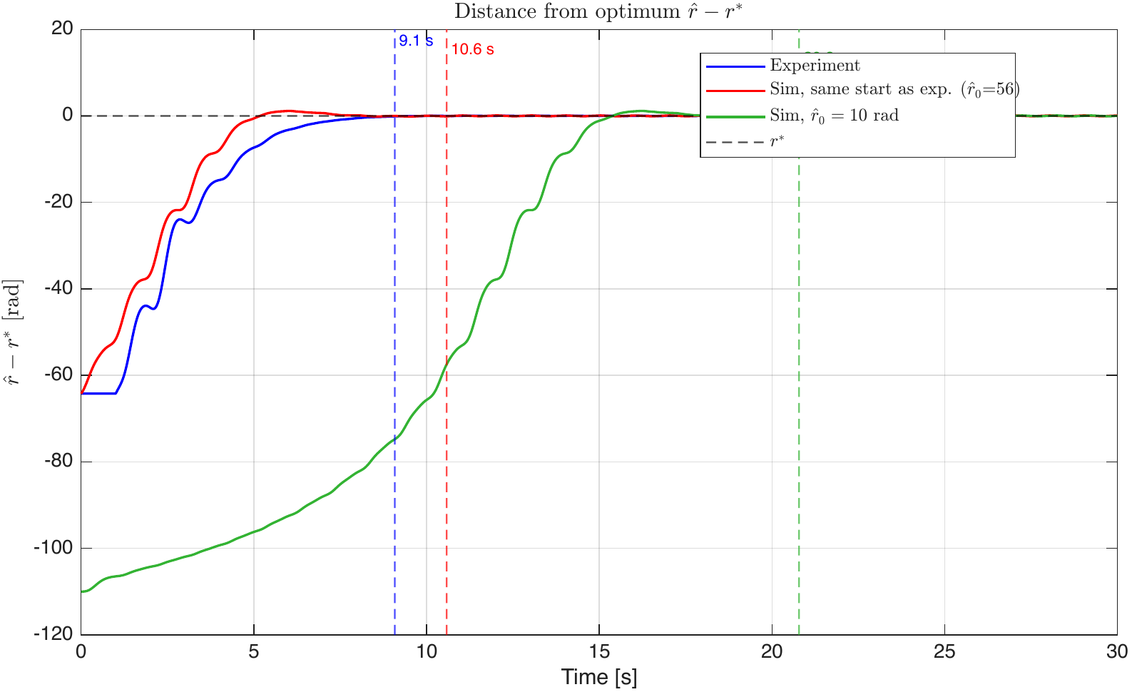
- Convergence speed: within 1.5 s of each other, validating the model
- Steady-state oscillations: smaller on the experiment ( vs. ), suggesting additional unmodeled HF attenuation
- Gradient estimate : less volatile in simulation, hinting at unmodeled plant dynamics
Positioning-Accuracy Trade-off (C-Q2)
A subtle but important effect: the actual position is , so even when has converged exactly to , the position still oscillates by around the optimum. If , the 0.1 rad positioning requirement is not met just by the nominal position alone.
Three levers affect accuracy:
- Reduce — smaller dither reduces oscillation but weakens the gradient signal (noisier , slower convergence)
- Reduce — less overshoot but slower convergence
- Reduce — better noise rejection but slower gradient extraction
This creates a fundamental convergence-speed vs. positioning-accuracy trade-off. For the dither-based accuracy requirement , both and must converge tightly to .
Moving Average ESC (C-Q3 & C-Q4)
The moving average (MA) filter replaces the HP → demodulation → LP chain with a single operation: averaging the demodulated signal over exactly one dither period .
The theoretical benefits are significant:
- Exact gradient extraction — the MA over one cosine period is exactly zero, perfectly canceling the dither component and all harmonics
- No phase lag — the classical HP/LP filters introduce phase lag ; the MA has only a fixed delay that is frequency-independent
- Simpler tuning — only the window length needs to match the dither period
- Higher dither frequencies possible — no strict timescale separation required
MA Simulation Results
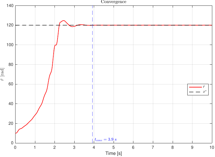
By exploiting the relaxed timescale constraint, the dither frequency was increased from to . The MA window shortened from to , enabling more aggressive tuning: , . Simulation convergence: 3.9 s — a 5× improvement over the classical approach.
MA Experimental Results
Seven runs on the physical setup. The best run (MA2: , , ) converged in 1.3 s — a 7× speedup over the classical experiment (9.1 s).
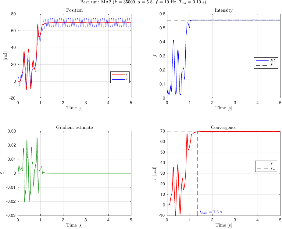
The MA approach proved sensitive to aggressive gain tuning: MA1 at went immediately unstable, showing the test setup has a lower maximum stable gain than simulation. Lower dither frequencies (2–5 Hz) converged significantly slower.
Classical vs. MA Head-to-Head
| Simulation | Experiment | |||
|---|---|---|---|---|
| Variable | Classical | MA | Classical | MA |
| Convergence time [s] | 10.6 | 3.9 | 9.1 | 1.3 |
| 0.549 | 0.540 | 0.555 | 0.556 | |
| oscillation [rad] | 0.09 | 0.03 | 0.03 | 0.06 |
Sampled-Data ESC (SD-Q1 → SD-Q4)
The sampled-data approach replaces the continuous sinusoidal dither with discrete step perturbations of amplitude and estimates the gradient via central differences:
where are steady-state intensity measurements at positions . A discrete-time integrator then updates: .
Three parameters govern SD performance:
- Step amplitude — finite-difference accuracy vs. signal-to-noise ratio
- Waiting time — must exceed the plant's settling time for unbiased measurements
- Step size — analogous to the integrator gain in classical ESC
Dither-Amplitude Analysis (SD-Q1)
- Small (< 0.5 rad): accurate finite difference, but is small relative to sensor noise → noisy estimates
- Medium (0.5–2 rad): good tracking, strong gradient signal
- Large (> 5 rad): overshoot + higher-order Taylor terms () degrade the approximation
SD Simulation Results (SD-Q3)
Tuned parameters achieved convergence in 8.7 s:
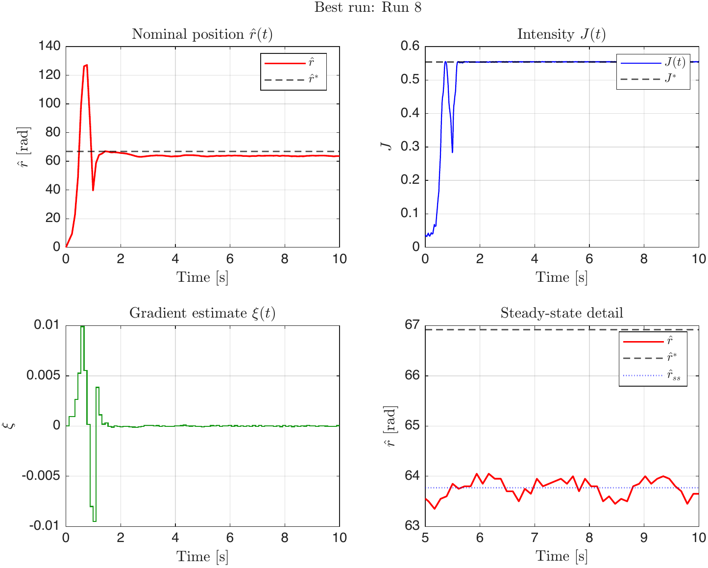
SD Experimental Results (SD-Q4)
Twelve runs were performed on the physical setup. None converged within the 0.1 rad bound due to a discovered implementation bug: the discrete-time integrator gain was set to instead of . The best run (Run 8) still settled to within 3.1 rad of the optimum.
Three-Way Comparison
| Approach | Best Experimental Convergence | Steady-State Accuracy | Tuning Complexity | MIMO Scalability |
|---|---|---|---|---|
| Classical | 9.1 s | < 0.1 rad | Moderate (, , ) | Poor (harmonic beating with dithers) |
| Moving Average | 1.3 s | < 0.1 rad | Moderate (, , , ) | Good (exact harmonic cancellation) |
| Sampled-Data | ~3 rad | Not met (bug in ) | Low (, , ) | Best (linear scaling with ) |
Key architectural differences:
- Classical: robust to noise (LP filter averages over many periods), but bound by
- Moving Average: exact dither cancellation enables higher frequencies and faster convergence, but sensitive to high gains and requires precise window matching
- Sampled-Data: simplest gradient estimation (only two measurements), naturally handles constraints via barrier functions, scales linearly to MIMO ( evaluations per iteration), but vulnerable to noise spikes on individual measurements
Engineering Takeaways
- Timescale separation () is the fundamental design constraint for classical ESC — it limits the achievable convergence speed but ensures filter stability. The MA filter relaxes this constraint and delivers order-of-magnitude speedups.
- Dither amplitude creates a fundamental trade-off: larger means better gradient SNR but more steady-state oscillation around the optimum. For the 0.1 rad accuracy requirement, itself must be < 0.1 rad.
- Simulation-to-hardware transfer is non-trivial: encoder offsets, unmodeled dynamics, and lower stability margins all required parameter re-tuning between simulation and the physical test rig.
- Implementation details matter: the sampled-data integrator gain normalization vs. was a subtle bug that made the difference between stable and unstable behavior on hardware.
Implementation Details
All three ESC approaches were deployed on the physical setup through MATLAB scripts that programmatically configure Simulink model parameters. The system sampling rate is .
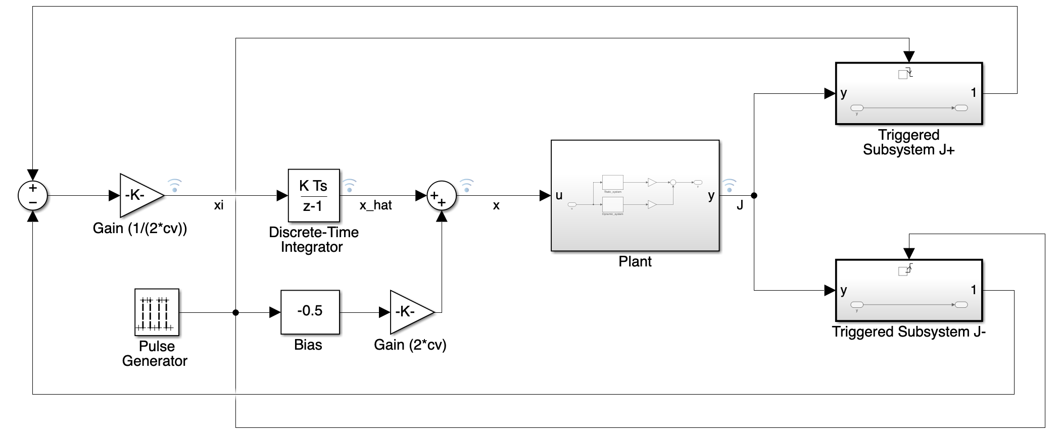
Classical / MA (ESC_CT.m)
The script toggles between classical and moving-average modes using gain switches, and discretizes the HP/LP filter prototypes before deployment:
% Classical ESC filter discretization
HPc = tf([1 0], [1 DE.highpass_filter_pole * 2 * pi]);
HPd = c2d(HPc, 1/Fs);
LPc = tf(1, [1 / (DE.highpass_filter_pole * 2 * pi) 1]);
LPd = c2d(LPc, 1/Fs);

% Toggle classical vs MA via gain switches
if DE.moving_average
    set_param(ModelName + "/DE/Gain_classic", "gain", "0")
    set_param(ModelName + "/DE/Gain_MA", "gain", "1")
end
For the MA filter, the FIR window length is samples.
Sampled-Data (ESC_DT.m)
The discrete-time implementation uses a pulse generator with period (one phase and one phase), triggered subsystems sample at the end of each phase, and a discrete-time integrator updates via forward Euler:
% Critical: integrator gain must account for sample time
set_param(ModelName + "/optimizer/Gain", "gain", ...
    num2str(optimizer.gain / (2 * dither.time)))
Objective-Function Measurement (linear_motion.m)
A linear sweep script ramps the stage position at constant velocity while recording encoder position and photodiode intensity. This produces a scatter plot of pairs that maps the lens-photodiode geometry — the source for the Q3 lookup table.
Technologies Used
MATLAB, Simulink, real-time hardware control, extremum seeking control, moving average filtering, sampled-data optimization, finite-difference gradient estimation, frequency-domain analysis (Bode plots, bandwidth), system identification, experimental parameter tuning